Formula

A SEI Formula is an Excel-like formula called NecAccess that, when called, can retrieve enterprise data from your databases.

SEI Formulas can be manually created or they can be easily generated using the SEI Formula Editor dialog window provided with the Excel Add-in.

The SEIFormulas work in the same manner as any other Excel function. They can be copied, pasted, and dragged from cell to cell. Performing these operations on a formula containing absolute or relative cell addresses will automatically adjust as required to the same extent that they would within a Sum function.

Exceptions to this rule are formulas that use the List operation. This type of operation which can affect cells adjacent to the active cell should not be automatically refreshed when recalculating a worksheet to avoid accidentally overwriting cells. As such, this type of formula is not saved into the cell as a regular Excel formula. It is saved into the cell as an Excel Cell Comment, which does not automatically get processed when refreshing the worksheet and is not an adjust cell when copied between worksheet cells.

To create a new formula using the SEI Formula Editor:

1. Click Formula Wizard in the Add-ins tab to open the SEI Formula Editor.
   

   

2. Select the Reference corresponding to the Data Model and the Environment you want to use to access the data you need.
3. Select the Field corresponding to the data to display with this formula.

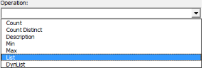
4. Select the Operation. There are many operations available:
   

   

   Operation	Description
   Count	To return the number of values for the selected field.
   Count Distinct	To return the number of distinct values for the selected field.
   Description	To specify that the selected field should actually return description type data.
   Min	To return the minimum value for the selected field.
   Max	To return the maximum value for the selected field.
   SUM	To return the sum value for the selected field
   SUM (Reversal)	To return the sum reversed for the selected value, could be used as an example for the sales revenue inside an income statement.
   SUM (Debit)	To return the sum value only if the total of the sum is a debit for the selected value.
   SUM (Credit)	To return the sum value only if the total of the sum is a credit for the selected value.
   List	To retrieve the list of values for the selected field. There are a few ways to display the list in Excel according to the choices made for list insertion method, list orientation and list ordering properties in the Setup window. This window shows up when the List option is selected as operation. Single Comma Delimited Cell: This is used to place the values into the current cell in a comma-delimited format. Replace Existing Cells: This is used to place the first value in the current cell and place the following values in adjacent cells while overwriting the content of those cells. Shift Existing Cells: This is used to place the first value in the current cell and the following values in the adjacent cells while shifting the content of those cells. Horizontal: To use the horizontal adjacent cells when placing the list values in many cells. Vertical: To use the vertical adjacent cells when placing the list values in many cells. None: No specific sorting order. Ascending: To sort the list in the ascending order. Descending: To sort the list in the descending order.
   DynList	To return the list of values for the selected field. The output is a comma delimited cell sorted in ascending order. The difference with the other list option is that this list will update as any Excel formula when the parameters are changed.

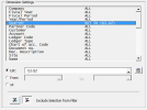
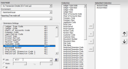
5. Specify the Dimension Settings by selecting the Dimension from the list of dimensions so that it gets highlighted then choosing one of the three filtering options available under the list area.

   Note

   This section is used to filter the records used within the calculations for the selected field and operation. You can enter those filtering settings for as many Dimensions as you like.

6. If you wish to filter values using a reporting tree node, select the reference cell you defined in Reporting Tree in the Reporting Tree node cell field.

   Note

   When you edit this field, the formulas are automatically refreshed.

7. In the List field, specify a list of values that should be included or excluded for the selected Dimension.

   • To determine if the values should be included or excluded, use the buttons Add Selection to Filter and Exclude Selection from Filter that show up when the List option is selected.

     

   • You can enter a unique value or a list of many values. You can manually enter values separated by a comma. For example, you can decide to exclude Quarters Q1 and Q2 by entering Q1, Q2 in the List field and by selecting the Exclude selection From filter button.

     

     You can also use wildcards to filter your values. Wildcards can only be used on text strings (not on numbers). Only one logic must be used at a time; for example, you cannot use 4?0*.

     • ? replaces one character

     • * replaces multiple characters

     

     Example of filtering values	Description
     4000	Single value
     4*	Must starts with 4
     4???	Must start with 4 and have a length of 4 characters
     4???-???-10	Must start with 4, followed by - and any 3 characters, followed by - and any 3 characters, must finish with 10, and must be 11 characters long

   • You can use the Prompt button next to the List field to select a range of values from the Prompt associated with the Dimension. In the Select List window that appears, you can select the values you want to include (or exclude) from the Available list (up) and use the Add Highlighted button to add them to the selected list (below). You can also Add All, Remove All or remove some values from the Selected List area (Remove Highlighted).

     

   • Using the Lookup button of the List field, you can get the value from an Excel cell, which can contain either one value, or multiple values separated by the default list separator.

   • In the From .. To field, specify a range of consecutive values to include to (or exclude from) the filter for the Dimension, the first one being entered or selected in the From: field, and the second one in the To: field. The way to enter values in each of those two fields is the same as for the List: field, as presented above.

   • Select All if you do not want to apply any filter for the selected dimension. This is the default value.

8. Click OK. The resulting SEI formula can be seen in the Excel formula bar.