Year Sparklines

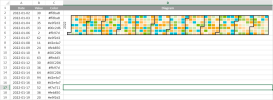
A year sparkline has 54*7 squares. The horizontal direction is the year week (from left to right, from 1st to 54th). The vertical direction is the weekday (from top to bottom, from Sunday to Saturday). The color of the days in the year depends on the value (from minimum to maximum, from startColor to middleColor to endColor).

To create year sparklines in the workbook:

1. Click Insert from the menu.

2. Click Sparkline and select the year sparkline under Calendar Sparkline from the list.

   

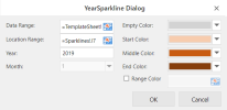
3. The YearSparkline dialog box is displayed:

   1. Set the parameters as described below.

   2. Click OK.

   

4. The sparkline is displayed in the cell. To edit the sparkline, click Design from the menu and select Settings. The YearSparkline dialog box will be displayed again.

5. Copy and paste the cell as needed to finalize your year sparklines.

   

Year sparkline parameter	Description
Data Range	The reference represents a range where the first column is a date and the second column is a number, such as 'A1:B400'.
Location Range	The cell where the year sparkline will be displayed.
Year	The full year number, such as 2015.
Month	The month number, such as 3.
Empty Color	The color string represents the days that have no value or zero value, such as 'light gray'.
Start Color	The color string represents the day where the value is the minimum value, such as 'light green'.
Middle Color	The color string represents the day where the value is the average of minimum and maximum, such as 'green'.
End Color	The color string represents the day where the value is the maximum value, such as 'dark green'.
Range Color	The reference represents a range where the data is a color string.
The year sparkline formula has the following formats: =YEARSPARKLINE(year, dataRange, emptyColor, startColor, middleColor, endColor) =YEARSPARKLINE(year, dataRange, colorRange)