Vbar Sparklines
To create vertical bar sparklines in the workbook:
-
Click Insert from the menu.
-
Click Sparkline and select the vbar sparkline under Bar Sparkline from the list.
-
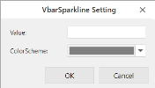
In the VbarSparkline Setting dialog box:
-
Enter the number or reference that represents the length of the bar, such as 0.3 or "A1".
-
Select the color scheme. The default value is "gray".
-
Click OK.
-
-
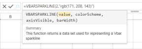
The sparkline is displayed in the cell. Click the function to edit the sparkline parameters.
-
Set the parameters as described below and click OK.
The vbar sparkline formula has the following format:
=VBARSPARKLINE(value, colorScheme, axisVisible, barWidth)
-
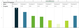
Copy and paste the cell as needed to finalize your vbar sparklines.
| Vbar sparkline parameter | Description |
|---|---|
| Value |
Number or reference that represents the length of the bar, such as 0.3 or "A1".
|
| colorScheme | String that represents the color of the bar; the default value is "gray". |
| axisVisible | (Optional) Boolean that represents whether to show the axis; the default value is true. |
| barHeight | (Optional) Number that represents the percentage of bar height according to the cell height (value > 0 and value <= 1). |
| barWidth | (Optional) Number that represents the percentage of bar height according to the bar width (value > 0 and value <= 1). |
| LET function |
(Optional) You can add a LET function to set colors according to specific values with IF statements. For example: =LET(ref,C3,color,IF(ref>=0.8,"#092834",IF(ref>=0.6,"#347B98",IF(ref>0.4,"#66B032",IF(ref>=0.2,"#B2D732",IF(ref>=0,"#F0F7D4","red"))))),VBARSPARKLINE(ref,color,TRUE,0.4)) |


