Pie Sparklines

To create pie sparklines in the workbook:

1. Click Insert from the menu.

2. Click Sparkline and select the pie sparkline under Pie Sparkline from the list.

   

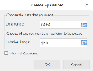
3. In the Create Sparklines dialog box:

   1. Select a range of cells in the same row or the same column.

   2. Select the cell where the sparkline will appear.

   3. Click OK.

   

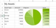
4. The sparkline is displayed in the cell. You can now customize the sparkline by clicking Design from the menu and selecting Settings.

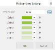
5. Set the parameters as described below and click OK.

   

6. Copy and paste the cell as needed to finalize your pie sparklines.

   

Pie sparkline parameter	Description
Percentage	If the parameter is a cell (such as: A1), the percentage is the cell's value. If the parameter is a range (such as "A1:B3"), the percentage is the result of each cell's value divided by the sum of the range. If the parameter is a percent value (such as 30% or 0.3), the percentage is the value. If the parse value is invalid, it will be treated as 0.
Color1 to Color5	Allows to define multiple colors based on this criteria: If the color parameter count is greater than or equal to the range count, values and colors have a one-to-to correspondence; redundant colors will be ignored. If the color parameter count is less than the range count, the given colors are reused and a linear gradient is used to ensure each sector has a different color. If there is no color, it uses "dark gray" as default.
The pie sparkline formula has the following syntax: =PIESPARKLINE(Percentage,color1,color2,.....)