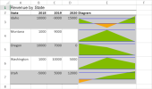
Area Sparklines
To create area sparklines in the workbook:
-
Click Insert from the menu.
-
Click Sparkline and select the area sparkline under Line Sparkline from the list.
-
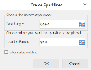
In the Create Sparklines dialog box:
-
Select a range of cells in the same row or the same column.
-
Select the cell where the sparkline will appear.
-
Click OK.
-
-
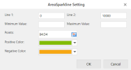
The sparkline is displayed in the cell. You can now customize the sparkline by clicking Design from the menu and selecting Settings.
-
Set the parameters as described below and click OK.
-
Copy and paste the cell as needed to finalize your area sparklines.
| Area sparkline parameter | Description |
|---|---|
| Line 1 | (Optional) A number that represents a horizontal line's vertical position; the line does not exist by default. |
| Line 2 | (Optional) A number that represents another horizontal line's vertical position; the line does not exist by default. |
| Minimum Value | (Optional) A number that represents the minimum value of the sparkline. The default value is the minimum value in the range. |
| Maximum Value | (Optional) A number that represents the maximum value of the sparkline. The default value is the maximum value in the range. |
| Points | It is a range, such as "D1:D6". If a cell value is not a valid number, it will be treated as 0. |
| Positive Color | A string that represents the color of the area in which the value is positive; the default value is "#787878" (RGB: 120, 120, 120). |
| Negative Color | A string that represents the color of the area in which the value is negative; the default value is "#CB0000" (RBG: 203, 0, 0). |
|
The area sparkline formula has the following syntax: =AREASPARKLINE(points, min, max, line1, line2, colorPositive, colorNegative) |
|


